
[bibshow file=library.bib key_format=cite]
[wpcol_1half id="" class="" style=""]
[/wpcol_1half]
[wpcol_1half_end id="" class="" style=""]
Background
When we have a satisfactory model for one neuron (see Integrate-and-fire section), we can think about modelling a network of neurons. By connecting them with synapses, network models are a powerful tool to understand brain dynamics and the origin of the electrical activity observed in vivo. The type of the neuron models used and the connectivity scheme influence the kind of dynamics that can be observed: in the following, we will focus mainly on recurrent networks of integrate and fire neurons. Among alternatives approaches, networks of binary neurons are easier to analyse analytically [bibcite key=Vreeswijk1996,Vreeswijk1998,Sompolinsky1988]. Those models treat the neuron like the spin of an elementary particle, its activity being a binary variable (spiking or silent), and established a link between theoretical physic and neuroscience. Models such as the Ising model [bibcite key=Schneidman2006,Marre2009] are used to infer correlations and structure of the neuronal code. Behind all these models, the key point is to explain the irregularity of the neuronal discharges observed in vivo. To explain it without stochastic inputs, one needs to have large fluctuations of the neuronal dynamics, counterbalanced by weak synaptic weights and by the fact that the activity should be balanced: an excitatory and and inhibitory population should act such that the average activity stays below a certain threshold, while fluctuations may be high and let the neurons cross a threshold, in order to emit spikes.
[/wpcol_1half_end]
[wpcol_1half id="" class="" style=""]
The balanced network
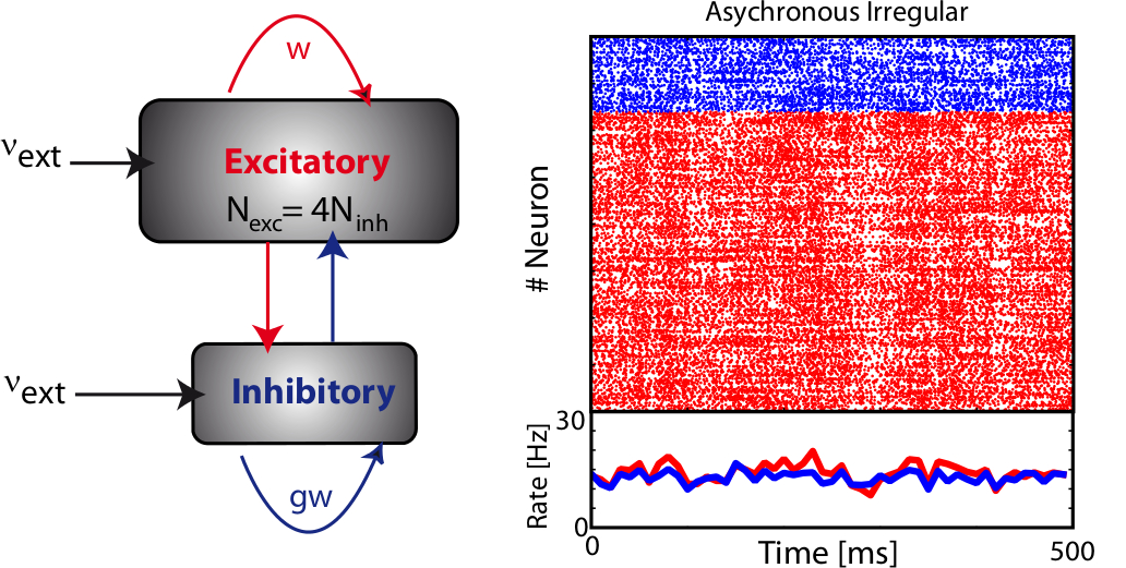
The balanced random network [bibcite key=Vreeswijk1996,Vreeswijk1998,Brunel2000,Vogels2005a,Kumar2008a,ElBoustani2009a,Amit1997,Renart2010] is a common and convenient framework for studying the dynamics of large-scale populations of sparsely-connected integrate-and-fire neurons. In these networks, two generic populations of excitatory and inhibitory neurons are reciprocally coupled with weights  and
and  (see Figure) to generate a balanced regime where the average depolarization of the neurons is roughly constant, subthreshold, and irregular spiking is the result of fluctuations. There is a classical ratio of 4 excitatory neurons for 1 inhibitory neurons, based on the measured ratio in cortex and a sparse, random connectivity. Every neuron is typically connected to
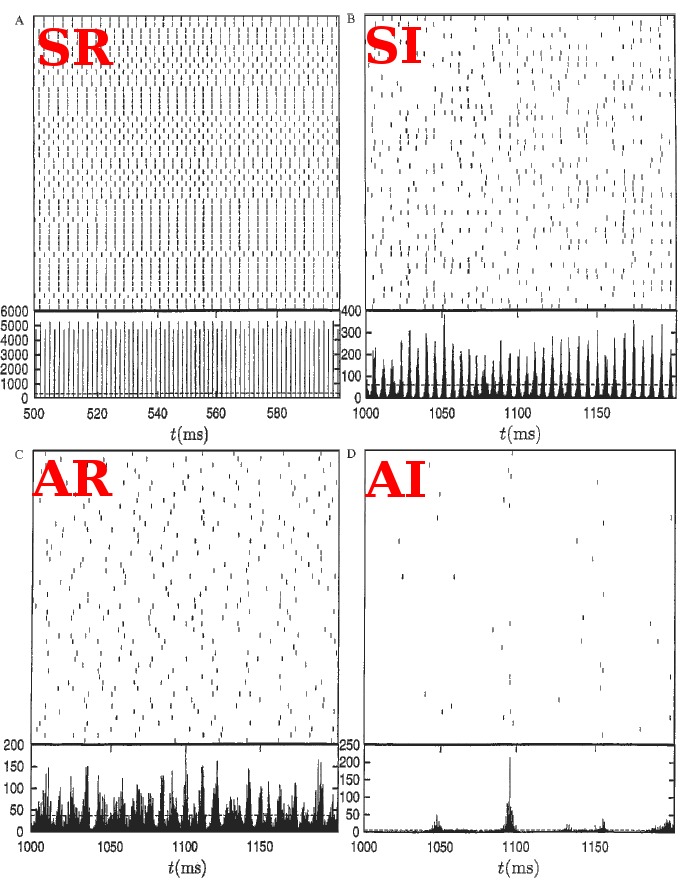
  of the others, and depending on certain key parameters, mainly the amount of external noise injected into the system and the balance between excitatory and inhibitory weights, several regimes of activity can be observed. Those regime have been described and classified in (Brunel, 2000), and can be asynchronous/synchronous (from a population viewpoint) and regular/irregular (from a neuron viewpoint).
[/wpcol_1half]
[wpcol_1half_end id="" class="" style=""]
[/wpcol_1half_end]
[wpcol_1half id="" class="" style=""]
[/wpcol_1half]
[wpcol_1half_end id="" class="" style=""]
Classification of the dynamics
The average firing rate of all the neurons within the network can be constant (asynchronous) or display oscillations (synchronous). The individual discharge of one neuron can be regular (the inter spike intervals (ISIs) are almost all equal), or irregular (the ISIs follow a Poisson distribution). This irregularity is often quantified by the coefficient of variation (CV), given by  where
where  denotes the average and
  the standard deviation. A pure Poisson process has a CV equal to 1. The more the discharge is regular, the more the CV tends to 0. Classical values observed in vivo in the spontaneous regime are usually close to 1, so simulations tend to focus on the irregular regime. In such a regime, neurons fire in an irregular manner, behaving almost like Poisson processes, and the average pairwise cross-correlation is modulated by the internal balance or the external input. This regime is also well suited to produce slow oscillations comparable with oscillations observed in vivo under anaesthesia [bibcite key=Han2008,Arieli1996]. Mean field models are a common tool used to establish and predict, analytically, the stationary average response of homogeneous networks of integrate-and-fire neurons under certain assumptions (neuronal discharges should be independent and Poissonian, in the irregular regime) [bibcite key=ElBoustani2009a,Brunel2000]. However, they are much harder to use when complex models of neurons are used, or when inhomogeneities, such as delays, are taken into account.
[/wpcol_1half_end]
[wpcol_1half id="" class="" style=""]
Mean field models
While the integrate-and-fire and compartmental models consider that the exact times of spike occurrence are important and may play a role in the coding strategies used in the cortex, other models consider that the pertinent information is in the instantaneous firing rate of the neuron. Since the discharge of the cell can be noisy and irregular, the spikes are not modelled and the only relevant information used by those models is the firing rate of the neuron. At each time, the neuron can emit spikes with a certain probability  , directly related to the activities
  of its pre-synaptic sources, weighted by some factors
  :
:
\begin{equation}
\frac{dr(t)}{dt} = \sum_i w_i f(r_i(t))
\end{equation}
where  is a positive, monotonic and increasing function, inducing a non linear relationship between the summed inputs and the instantaneous firing rate . Usually, is a sigmoidal or a hyperbolic tangent function. An alternative viewpoint is to say that
  represent the average firing rate over a population of identical neurons, rather than an instantaneous frequency, and that is why these equations are called mean-field or rate-based models. Solid mathematical results can be obtained with these mean field models, concerning either their dynamics or their learning properties.
[/wpcol_1half]
[wpcol_1half_end id="" class="" style=""]
[/wpcol_1half_end]